Research
22 pages
Combining direction and volatility forecasts of stock market returns
On this page
Volatility models are mostly endogenous: they exclude macroeconomic variables because the frequencies do not match — prices arrive daily, macro data monthly at best. GARCH-MIDAS solved the frequency problem but still ignored regime switching, even though bull and bear markets plainly have different unconditional volatility.
This dissertation adds macro-driven regime switching to GARCH-MIDAS, predicts the market state exogenously rather than inside the model, and lets duration affect the switch probability non-linearly. It also asks whether the March 2020 collapse and recovery were predictable from macro variables at all.
The full text is below, typeset from the original LaTeX. Both language versions are available as PDFs.
In this paper I extend GARCH-MIDAS model to include macro-based regime switching. I examine effects of macro-variables on predicted state and volatility of the market. The market regime forecasting is augmented with non-linear duration dependence. I also suggest a new method for market regime identification. Empirical results confirm findings of previous works and demonstrate significant improvement in volatility forecasting accuracy.
Introduction
Market volatility forecasting has long been an issue in financial literature due to its use in option pricing and various risk metrics. Yet, most volatility models are endogenous and do not include external variables, especially, the macro ones due to mismatch in frequency: market prices are available at almost arbitrary frequency, while most macroeconomic variables are at best have weekly frequency but more often it is monthly or quarterly. At the same time financial volatility as noted by several researchers (see Literature Review section) has roots in real economy and fundamental uncertainty. In drawing such conclusions those authors have employed market data at monthly frequency, which makes these results hardly useful for practitioners.
The situation has changed with introduction of the new GARCH-MIDAS type models, which allowed for incorporation of different frequency data in volatility models. Such models have proved to be superior to standard types yet they still lacked an important feature that has been widely documented in past research - regime switching in market volatility. Bull and bear states of the market have different unconditional volatility. Except a single attempt to incorporate regime-switching in the GARCH-MIDAS framework (Pan et al., 2017) the issue has not yet been thoroughly addressed. Moreover, in that work probability does not include some important features such as duration dependence. In this paper I present the regime-switching GARCH-MIDAS model, where market regime is predicted with macro-variables. I compare this model with non-regime-switching one and find that the former significantly outperforms the later.
The second aim of this paper is to examine regime forecasting on the new data. In the spring 2020, when all the real economy indicators showed sharp declines, the stock market seemed not to notice the global economic downturn. Various explanations were proposed, yet no formal model could explain the apparent discrepancy. From the general prospective, stock prices are directly based on the real economy: a single share derives its value from future dividends (discounted at a proper rate), dividends are paid based on firm's profits and profits is a reflection of the firm's performance, i.e. its contribution to the value added of the economy. Thus, it might seem obvious that the stock market must reflect changes in the real economy. Yet, the data indicates that the relation between real and financial sectors is rather indirect, although there is no doubt that in the long run all the financial assets will end up in the real economy. Hence, I want to examine whether the market decline of March 2020 and subsequent recovery was predictable based on macro variables and whether it goes in line with them. Another minor contribution of this work is incorporation of non-linear duration dependence in the market state dynamics.
There are several reasons why one would be interested in forecasting market state. First, it is essential for investors and fund managers to employ market-timing strategy - switching from risky to risk free assets depending on the state of the market. Second, it would be of use to the policy makers to plan financial stability control measures.
The paper is organiszed as follows: in section 2 I present the literature review with focus on recent advancement in market state and volatility forecasting models, in section 3 I present the econometric framework where I combine the two, in section 4 I provide estimation results based on numerical optimization and section 5 concludes the paper.
Literature review
This literature review section will be divided into two parts. In the first one we consider the research on predictability of stock market regime. In the second one we consider the existing models of market volatility forecasting.
Determining and forecasting the direction
Over the past 3 decades the consensus on what exactly to call bull and bear markets has not yet been reached. Usually we can find general definitions like "prolonged periods of decreasing and increasing market prices" (Chauvet and Potter, 2000). Most authors employ some variation of the former but there are also stricter wordings. For example, Sperandeo (1990) defines market regimes in more exact terms: "A long-term upward/downward price movement characterized by a series of higher/lower intermediate highs/lows interrupted by a series of higher/lower intermediate lows/highs", which is essentially corresponds to the definition of trend in technical analysis. The problem with this kind of definitions, as I will discuss later, is that they implicitly imply forward-looking determination of current state (current state depends on whether the next high/low will be higher or lower of the previous high/low). Therefore, short horizon predictions are not possible. In this paper we will understand bull / bear markets as an average positive / negative return of the market, respectively.
Despite the research on identification of bull and bear markets have attracted more interest over the last two decades, it is still rather limited. The two main approaches that can be found in literature are Markov-switching parametric approach and a semi-parametric one. The Markov-type models have an advantage also highlighted by Kole and van Dijk (2017) that such models specify a single data-generating process that can be used as for identification of the regime as for forecasting, while semi-parametric models would require an additional step of parametric forecasting. Kole and van Dijk (2017) conduct a comparative study of Markov-type and semi-parametric models and come to the conclusion that semi-parametric models work best for in-sample prediction and Markov-type models work best for in-sample prediction. The reason is that Markov-switching models account for volatility while semi-parametric ones only consider mean return.
The regime switching Markov model has been widely used in sorting out market states. The starting point of research is Hamilton (1989), who proposes a specification of Markov switching model, which endogenously sorts market into regimes and allows for time varying conditional mean and variance. Maheu and McCurday (2000) incorporate duration dependence in the model, that is probability of regime switch depends on duration of regime at a time. They report volatility in the bear state is an increasing function of duration. In the bull state returns are an increasing function of duration, that is the probability of observing the end of positive returns series will decline with duration.
Semi-parametric approach is different to Markov regime-switching one in that we separate identification and forecasting. That is why the approach is called semi-parametric. First, we perform non-parametric identification and second, we construct a binary choice predictive model. As the two steps are unrelated, we consider them one by one.
There are several major methodologies to distinguish market into regimes non-parametrically. Originally that was an issue in business cycle modeling to identify recessions and contractions in the real economy. Later on some of those techniques were employed in sorting out market regimes. For example, the well-known Bry and Boschan (1971) algorithm also used in Nyberg (2013). This approach incorporates a combination of two Moving Averages, a Spencer curve1 and various filtering procedures. Nyberg (2013) shows the market state to be predictable more than market returns on a 1 to 12 months forecasting horizon. He uses typical dataset for such studies: SP500 as a market proxy, treasury market yields (term structure yield spreads, federal funds rates, constant maturity yields), unemployment rate, industrial production, and inflation. Again, term structure yield spread appeared to be the most significant predictor. The main contribution of his work is incorporation of dynamics into the previously static probit models. That resulted in significant improvement of forecasting accuracy with term spread being the most significant predictive variable.
The two similar and widely used approaches in market regime identification were those proposed by Pagan and Sossounov (2003) and Lunde and Timmerman (2004). Those two will be later referred to as PS and LT, respectively. The PS rule-based identification procedure requires the state (bull or bear) to have a certain duration and magnitude of price changes while LT only considers the amplitude. As LT put it,
"...the stock market switches from a bull state to a bear state if stock prices have declined by a certain percentage since their previous (local) peak within the bull state."
A one drawback of this approach is that it employs a forward-looking parameter2. Therefore, it will have a time lag (usually, a substantial one), which makes it not quite useful in out-of-sample prediction. The forward looking determination of cycle is more reliable and can be really useful in business cycle analysis but we cannot afford it in market state determination because changes in trend can happen withing the days. For example, the S&P500 market index fell from 3393 on 16/02/2020 to 2280 on 15/03/2020. A total loss of 32% within a month. Hence, the speed of adjustment is crucial here.
Interestingly, Lunde and Timmerman (2004) mention the use of technical rule in determining market trends3, saying the restriction of time horizons in such rules are rather short. As I have mentioned earlier, trends may indeed be quite short such as the one in February - March of 2020, and yet it was a rightful economically reasoned trend. This is a crucial point since many authors follow an assumption of a particular minimum duration of market phase. For example, both Nyberg (2013) and Chen (2009) as well as Candelon et al. (2008) employ a restriction of minimum market state duration of 6 months. Clearly, such kind of restriction would limit our ability to identify market movements at higher frequencies, such as market declines of 2016 or 2018.
As an identification procedure Chen (2009) examines what he calls a naive approach. He uses the simple moving average of stock returns with a fixed smoothing period4. When the average return over  periods is positive we assume the state of market in the given period to be bullish and when average return is negative the market is said to be bearish. He finds no significant difference in forecasting accuracy when switching from Markov-type model to semi-parametric with naive identification. His findings suggest that inflation and interest rate spread are the most significant predictors of market state, while monetary aggregates and exchange rates appeared to be poor predictors.
Generally, all the authors employ similar dataset and with different methodologies and approaches come to similar conclusions: market state is more predictable than market returns with interest rate spread being the most useful predictor.
Volatility forecasting
Whereas in case of market regime the most complex part was to identify the regime in an unambiguous and consistent way, market volatility (realized volatility) is directly observable (squared returns) and the most attention is given to forecasting procedures. We can probably start the review of literature on the topic from Schwert (1989), though there were some earlier works such as Officer (1973). Schwert (1989) examines effects of various macroeconomic variables including inflation, base rate, financial leverage and monetary aggregates as well as their variances on stock market volatility. Most of coefficients were positive and some were reliably above zero. Financial leverage appeared to have low effects. Schwert (1989) shows that returns of financial assets are more volatile during recessions in real economy, which is explained by the effect of operating leverage. Financial volatility originates in real economy but there is weak evidence that macroeconomic volatility can predict that of financial market. Later authors, however, advanced in sophisticated forecasting models that have proved the opposite.
Engle and Rangel (2008) introduced a Spline-GARCH model, where variance consists of two components: a deterministic one and a mean reverting unit daily GARCH. Such a distinction allowed for time varying unconditional variance. Engle and Rangel find that volatility in macroeconomic factors (they employ GDP growth, inflation, and short-term interest rates) are important explanatory variables of stock market volatility. Engle et al. (2013) go further and suggest an improvement over spline-GARCH, which allows to account for economic roots of financial volatility. They return to the question raised by Schwert, namely why does volatility changes over time?. They conduct a study of long-run volatility over the 1884-2010 period of the US market using the more advanced tool of GARCH-MIDAS model. It allows the long-term volatility component to be a function of macroeconomic variables. Engle et al. (2013) limit macro variables choice to inflation and industrial production growth. They confirm findings of Engle and Rangel (2008) regarding effect of macro variables: "industrial production and inflation account for roughly between 10% and 35% of expected one-day-ahead volatility". Concerning predictive ability of the new model class, GARCH-MIDAS "is roughly at par with time series volatility models at the quarterly horizon and at par or outperforms them at the semiannual horizon".
The most attractive feature of the GARCH-MIDAS model is that it allows for different frequencies of the time series. Such a feature is really useful in macro-financial analysis because most of macro-variables are monthly to quarterly prices while the price data is available at daily frequencies. The MIDAS (Mixed Data Sampling) approach, originally introduced by Ghysels et al. (2006), allows us to decompose variance into long-term and short-term components, where macroeconomic variables would be responsible for long-run volatility while mean reverting unit daily GARCH for the short-run one.
Asgharian et al. (2013) slightly modified the setup of Engle et al. (2013) by including both smoothed realized returns volatility and macroeconomic data (both level and variance) in the long-term volatility component. They report improved forecasting accuracy over the standard GARCH-MIDAS model. They use US market data for the 1991-2008 period and find the short term interest rate to be the most significant explanatory variable.
An extension to GARCH-MIDAS model was suggested by Pan et al. (2017). They allowed for regime switching in volatility governed by Markov transition matrix. The classical GARCH models without structural breaks can result in spurious volatility persistence. Therefore, regime switching is a crucial aspect in drawing accurate predictions especially given significant empirical evidence of significantly different volatility in bull and bear states. In this paper I am employing volatility regime switching as in Pan et al. (2017) but also introduce switch in mean return, which is natural but was omitted in Pan (2017). I also forecast probabilities exhogenously rather than within the model.
Econometric framework
Here I will present the formal model to be estimated. In direction determination and forecasting I combine approaches of Chen (2009), Nyberg (2013) and Maheu and McCurdy (2000). In volatility forecasting I essentially use framework of Asgharian et al. (2013). Finally I combine the two similarly to Pan et al. (2017) but with different regime probability process and certain other extensions.
Determining direction
The simplest way to sort out the market regimes is to use simple moving average of stock returns with smoothing period  :
:

When the average return over periods is positive we assume the state of the market in time  to be bullish and when it is negative the market is said to be bearish. We can also use weighting scheme here and/or apply a combination of moving averages. For example, we can use
  to determine the bull market. Those are classical tools of technical analysis, yet rarely used in scientific literature.
The advantage of using such indicators is that they are first, not forward-looking (and hence can be used for out-of sample prediction) and second, have a straightforward calibration of parameters. Here I take an Exponential Moving Average (EMA), which gives more weight to recent values and hence would be more responsive to trend reversal:

, where  is a smoothing constant (usually, 2) and is number of smoothing periods. As we increase , EMA will capture larger price movements while disregarding the smaller ones. Lower value of would correspond to higher number of identified regimes, which will be shorter in duration.
Forecasting direction
From here we treat the market state  as observable with
  corresponds to the bear state and
  to the bull sate. We begin with the basic binary choice framework, where the prediction probability of market being in a bull state in
  periods from now is give by
 (1)
(1)where  is a macroeconomic variable and
  is a cumulative probability distribution function. For the out-of-sample forecasts evaluation I use the quadratic probability score:
 (2)
(2)with the score of 0 corresponding to the 100% accuracy, while the maximum value of 2 means complete failure.
Such a specification only includes one explanotary variable and lacks several other important features. Let is first introduce a linear function for market state of explanotary variables as
 (3)
(3)where  is a vector of explanatory variables and
  is the one of coefficients. Now,
 (4)
(4)We can also include the lagged value of market state as
 (5)
(5)Maheu and McCurdy (2000) among others highlight the significant variations between bull and bear market duration. Indeed, bull markets tend to be more prolonged and less volatile than the bear ones. Therefore, it might be reasonable to include the duration in the equation. Maheu and McCurdy (2000) define duration as
 (6)
(6)We also would like to capture non-linearities in duration dependence. We would expect the duration of trend to increase  in the beginning and to decrease as the trend continues. Hence we need a non linear structure to account for such dependence. We use the quadratic structure. Moreover, as dependence is expected to be different for bull and bear markets we distinguish between two.
 (7)
(7)We might reasonably expect that duration of each state would converge to some mean value over the long run. That is the persistence of market state. Thus, the probability of next state to be the same as the previous one can be expected to have concave parabolic dependency on its duration. I then expect signs of  to be positive and of
  to be negative. Signs of
  and
and  are expected to have the opposite signs (as we essentially forecast probability of the bull market) - negative and positive, respectively.
Forecasting volatility
We now proceed to a formal GARCH-MIDAS framework (see, for example, Engle et al. (2013) or Asgharian et al. (2013)). Return  in month
  , day follows the following process:
 (8)
(8), where  is the short term component of the volatility and
  is the long term one. follows the daily GARCH(1,1) process:
 (9)
(9)I now introduce regime switching both in mean and variance. First, I say mean return is now time-varying and contingent on current market regime:  . Similarly we redefine
 (10)
(10)The  component (unchanged) is defined in the spirit of MIDAS regression:
 (11)
(11), where RV is realized volatility
 (12)
(12),  is the exponential weighting scheme5
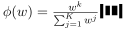 (13)
(13)and K is the number of periods of smoothing. The total conditional variance is defined as
 (14)
(14)The equations (9) to (13) constitute the GARCH-MIDAS model with the parameter space  .
.
Asgharian et al. (2013) also suggest incorporating macroeconomic variables and their volatilities directly to equation (11).
 (15)
(15), where  is the level of macroeconomic variable and
  is its variance. Asgharian et al. (2013) do not use the exponent but Engle et al. (2013) argue it is needed to ensure long run volatility is positive.
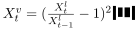
Similarly to volatility of stock market returns, we define as
 (16)
(16)Following Asgharian et al. (2013) we use an estimation window of 10 years and and perform an ou-of-sample test with constant parameters for the subsequent year.
Combining the two approaches
There is significant evidence of volatility being state dependent (see for example Kole and van Dijk (2017), Maheu and McCurdy (2000), Lunde and Timmermann (2004), Schwert (1989), Marcucci (2005)). Bull markets usually tend to be long and low volatile, while bear markets are usually short and highly volatile.
As in Pan et al. (2017) we introduce conditional distribution vector  :
:
 (17)
(17), where is a normal distribution function.
Thus, without regard to market state,
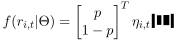 (18)
(18), where  - probability of bull state in the next time period - is assumed to be exhogenously given. Its forecasting is described in section 4.2. An important contribution of this paper can be seen here: while traditionally GARCH-MIDAS models only incorporate low-frequency data to forecast long-term volatility component and model short-term volatility dynamics as daily GARCH(1,1) process, I also include daily-frequency data into the forecast of the next state probability.
Now let is write down the return distribution function explicitly:
 (19)
(19)From here we can construct the Maximum Likelihood estimator
 (20)
(20), from where we get  .
.  here represents number of months and
  is the number of days in month .
We also would like to estimate standard errors. The standard procedure (Pan et al., 2017) involves estimation of covariance matrix from the Hessian. If we denote Hessian  , covariance of log-likelihood scores
  , scalar step size
  and vector
  , where all element except for are zeroes, then covariance matrix
  can be estimated as follows:
 (21)
(21)Derivative is approximated as
 (22)
(22)and is given as
 (23)
(23)After the above have been calculated, standard errors are constructed in a standard way:
 (24)
(24)Data
All the data I use was obtained from FRED 6 for the period January 2003 to April 2021. The inflation is constructed as monthly percentage change in CPI. In the similar way I got market return. Here I have used the Wilshire 5000 index instead of commonly used S&P500 or NASDAQ for the reason that Wilshire 5000 includes all US traded stocks (For the time being this number is 3141) and therefore it is more representative indicator of economic activity, although it is almost perfectly correlated with S&P500. Also I distinguish between daily and monthly data: daily data will be used to forecast market direction, while monthly data will be used in the long term component of volatility process.
In daily-frequency data we have
BRENT7: Crude Oil Prices: Brent - Europe
TBY2: 2-Year Treasury Constant Maturity Yield
TBY10 10-Year Treasury Constant Maturity Yield
TBY30: 30-Year Treasury Constant Maturity Yield
BEINF: The breakeven inflation rate8
MARKET: Return of market index
It is worth noting that I incorporate term structure of interest rates by including spot rates rather than spread as most authors do. As we will see later that does not really matter.
Table 1: Descriptive statistics of daily data
![{@{\extracolsep{5pt}}lccccc} \\[-1.8ex]\hline \hline \\[-1.8ex] Statistic & \multicolumn{1}{c}{Min} & \multicolumn{1}{c}{Mean} & \multicolumn{1}{c}{Median} & \multicolumn{1}{c}{St. Dev.} & \multicolumn{1}{c}{Max} \\ \hline \\[-1.8ex] BRENT & 9.12 & 69.60 & 64.31 & 27.38 & 143.95 \\ TBY2 & 0.09 & 1.6](/assets/papers/bsc-forecasts/en/d417d039e177d428.svg)
We also have variables sampled at monthly frequencies. Those are macroeconomic variables used in long-run volatility component of GARCH-MIDAS model. As a common convention, we take the first differences.
INF: Month to month percentage change in CPI.
INDPOROD: The Industrial Production Index is an economic indicator that measures real output for all facilities located in the United States manufacturing, mining, and electric, and gas utilities.
RETSALES: Retail and Food Services Total Sales, Millions of Dollars
UNRATE: Unemployment rate.
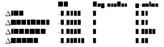
Table 2: Descriptive statistics of monthly data
![{@{\extracolsep{5pt}}lccccc} \\[-1.8ex]\hline \hline \\[-1.8ex] Statistic & \multicolumn{1}{c}{Min} & \multicolumn{1}{c}{Mean} & \multicolumn{1}{c}{Median} & \multicolumn{1}{c}{St. Dev.} & \multicolumn{1}{c}{Max} \\ \hline \\[-1.8ex] $\Delta$INF & $-$1.77 & 0.16 & 0.19 & 0.31 & 1.38 \\ $\Delta$INDPR](/assets/papers/bsc-forecasts/en/7e31429ded224795.svg)
The ADF tests for stationarity are presented in the appendix.
Now we would also like to consider statistics on bull and bear states. For example, let is examine durations of each state with EMA(30) used to distinguish between states.
Table 3: Descriptive statistics: market regimes duration
![{@{\extracolsep{5pt}}lccccccc} \\[-1.8ex]\hline \hline \\[-1.8ex] Statistic & \multicolumn{1}{c}{N} & \multicolumn{1}{c}{Mean} & \multicolumn{1}{c}{St. Dev.} & \multicolumn{1}{c}{Min} & \multicolumn{1}{c}{Pctl(25)} & \multicolumn{1}{c}{Pctl(75)} & \multicolumn{1}{c}{Max} \\ \hline \\[-1.8ex] Bull &](/assets/papers/bsc-forecasts/en/68117a5514b7a40d.svg)
From here we can already see that bull states tend to be on average twice as long as the bear states. But we would also perform the standard t-test for difference in means:
Table 4: Test for bull and bear equal regime durations
![{ c c } \\[-1.8ex]\hline \hline \\[-1.8ex] t & 5.5779\\ df & 395.75\\ p-value & 4.519e-08\\ \hline \\[-1.8ex]](/assets/papers/bsc-forecasts/en/a0ad919630cbe068.svg)
We also consider returns characteristics of bull and bear market:
Table 5: Descriptive statistics: returns in different market regimes
![{@{\extracolsep{5pt}}lccccccc} \\[-1.8ex]\hline \hline \\[-1.8ex] Statistic & \multicolumn{1}{c}{N} & \multicolumn{1}{c}{Mean} & \multicolumn{1}{c}{St. Dev.} & \multicolumn{1}{c}{Min} & \multicolumn{1}{c}{Pctl(25)} & \multicolumn{1}{c}{Pctl(75)} & \multicolumn{1}{c}{Max} \\ \hline \\[-1.8ex] Bull &](/assets/papers/bsc-forecasts/en/3cbefe3613df3733.svg)
Now we are mainly concerned with difference in variance, although difference in means should also be tested to meet requirements of bull and bear states definition. But even now we can see that standard deviation of returns in Bear state is on average twice as large as in Bull state.
Table 6: Test for equal mean return in different regimes
![{ c c } \\[-1.8ex]\hline \hline \\[-1.8ex] t & 19.708\\ df & 3135.8\\ p-value & <2.2e-16 \\ \hline \\[-1.8ex]](/assets/papers/bsc-forecasts/en/2a7380f10b8d9c14.svg)
And we also test bull and bear returns for equal variance with two-sided alternative:
Table 7: Test for equal variance of returns in different regimes
![{ c c } \\[-1.8ex]\hline \hline \\[-1.8ex] F & 0.34828\\ df1 & 4405\\ df2 & 2287\\ p-value & <2.2e-16 \\ \hline \\[-1.8ex]](/assets/papers/bsc-forecasts/en/391775619a4c2f7c.svg)
Empirical results
We begin with sorting market into states. Figure 1 shows periods of bear market with pink. As one can see the major bear periods correspond to the 2008 Global Financial Crisis, 2010 European Debt Crisis, 2016 market selloff, 2018 raise of rates by the Federal Reserve and the 2020 Covid shock.
Figure 1: Non-parametric market regime identification with EMA(500)
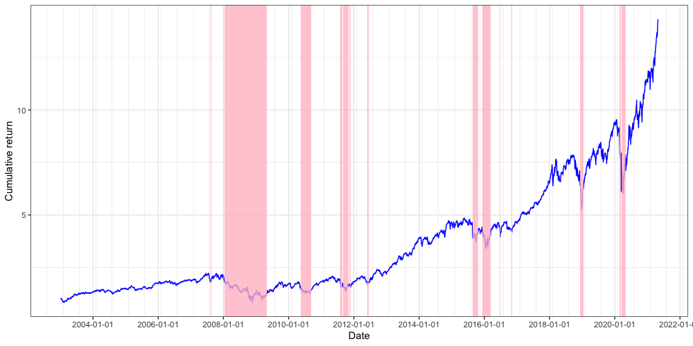
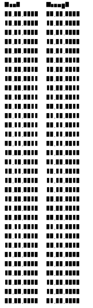
The full list of peaks and troughs is presented in the appendix.
First, we consider estimation results of direction forecasting model.
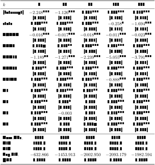
Table 8: Direction forecasting: probit estimates by horizon (days)
 ,
,  ,
,  ,
, 
For simplicity here I introduced the following notation: D1 =  , D2 =
  , D3 =
  and D4 =
  . From here it can be seen that the model works best for short-term predictions. The results above confirm significant predictive ability of the yield curve data. Based on QPS score short term forecasting under the considered model is the most accurate. Non-linear duration dependence has also proved significant for all except 30 and 90 days forecasting horizons. As could be expected, crude oil price negatively affects probability of bull market. Interestingly enough, the yield curve coefficients tend to sum up to 0, which means that we essentially use two term spreads: (TBY10 - TBY2) and (TBY30 - TBY10).
One should be very careful interpreting estimated duration dependence parameters. First, it can be noted that my initial expectation of parameters signs proved wrong with all the values being positive. This, however, confirms findings of Maheu and McCurday (2000) regarding persistence in market state: the longer is the bull market, the less likely it is to end. But the interpretation is different for the bear market: the longer is the bear market (parameters D3 and D4), the higher is the probability of switching to the bull one. Thus, while bull market have positive duration dependence, the bear markets essentially have a negative duration dependence.
Figure 2: Forecasted probability of bear market on different horizons
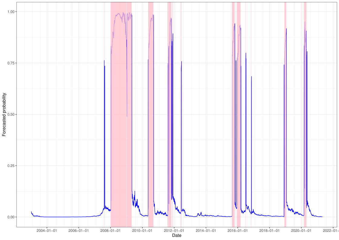
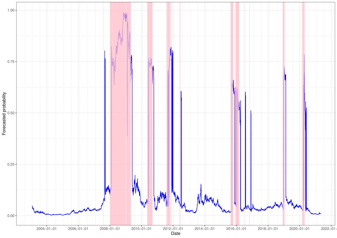
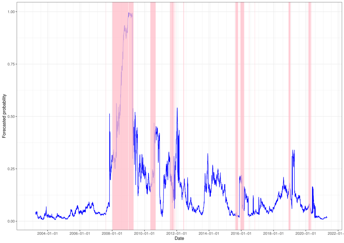
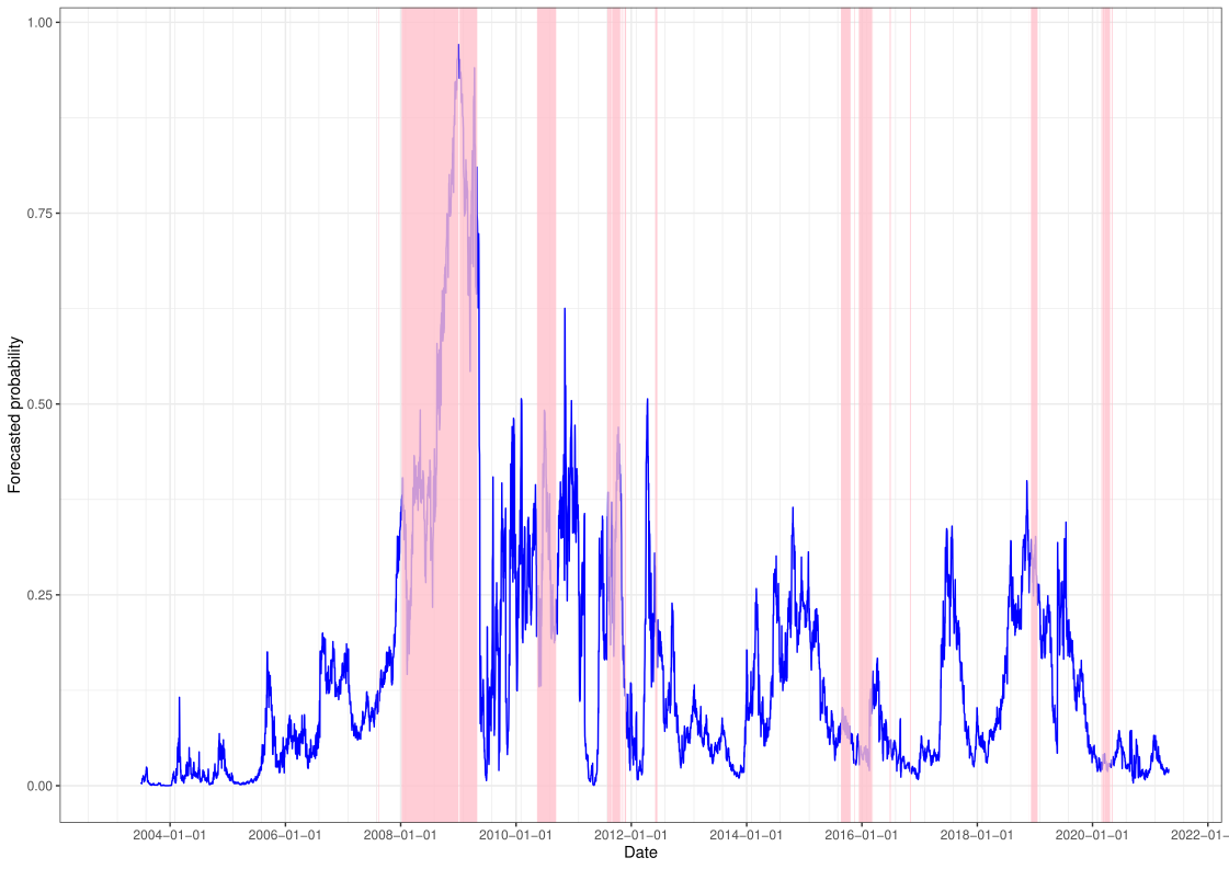
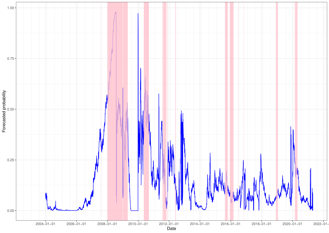
If we say that a bear market was predictable if its forecasted probability was above 0.5 (though, other thresholds can be used) than concerning 2020 market crash only 5 and 30 days ahead forecasts were accurate. On longer horizons the fall was unpredictable under the examined models.
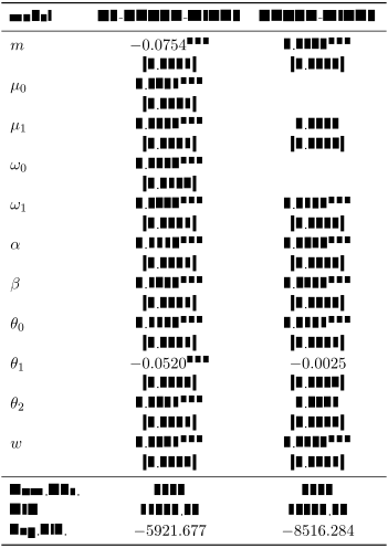
Now consider the maximum likelihood estimation of regime switching GARCH-MIDAS together with standard benchmark.
Table 9: Maximum likelihood estimates: regime-switching GARCH-MIDAS against the standard benchmark
, , ,
Based on the Akaike information criterion AIC the model with regime switching significantly outperforms the standard GARCH-MIDAS. The  and
and  components, which essentially account for macroeconomic information appear insignificant in the benchmark model but become significant with the regime switching one. It is worth noting the signs of parameters: market volatility and macroeconomic volatility (represented by
  and , respectively) positively affect forecasted market volatility, which is natural, while the level of macro-variable (retail sales first difference) is negatively associated with forecasted market volatility. As could be expected the unconditional long-term volatility component
  is greater for bear markets than for bull ones while the unconditional mean return
  is greater for bull markets. Thus, the model meets distinction between bull and bear markets discussed in the beginning and confirms findings of previous works.
Conclusion
In this paper I have analyzed existing models on direction and volatility forecasting of stock market returns. On the basis of previous research I have suggested an extension to the standard GARCH-MIDAS model by augmenting it with macro-based forecast of market state. Empirical results prove previous research conclusions of the significance of yield curve data for forecasting market direction. Moreover, non-linear duration dependence in direction forecasting has also proved to be highly significant for most prediction horizons. Bull markets tend to have positive duration dependence while Bear ones tend to have negative. This confirms findings of previous studies. Short-term (5 days ahead) forecasting appeared to be the most accurate. My findings suggest 2020 market crash was predictable one month before the actual fall but not predictable on the longer horizons. Inclusion of macro-based regime-switching in the GARCH-MIDAS resulted in significant improvement of forecasting accuracy.
The main contributions of this work are inclusion of macro-based regime switching in the GARCH-MIDAS model, regime forecasting on the new data, incorporation of non-linear duration dependence in market state forecasting, suggesting new method for market regime identification.
References
Asgharian, H., Hou, A. J., & Javed, F. (2013). The importance of the macroeconomic variables in forecasting stock return variance: A GARCH-MIDAS approach. Journal of Forecasting, 32(7), 600-612. https://doi.org/10.1002/for.2256
Chen S., 2009, Predicting the bear stock market: Macroeconomic variables as leading indicators, Journal of Banking & Finance
Cohrane J. H., 1991, Production-Based Asset Pricing and the Link Between Stock Returns and Economic Fluctuations, The Journal of Finance
Demir C., 2019, Macroeconomic Determinants of Stock Market Fluctuations: The Case of BIST-100, Economies
van Dijk D. and Cakmakl C. , 2016, Getting the most out of macroeconomic information for predicting excess stock returns, International Journal of Forecasting
Engle R. F., Ghysels E., and Sohn B., 2013, STOCK MARKET VOLATILITY AND MACROECONOMIC FUNDAMENTALS, The Review of Economics and Statistics
Ibbotson R. G.& Chen P., 2019, Long-Run Stock Returns: Participating in the Real Economy, Financial Analysts Journal
Kole, E., and van Dijk, D. (2017) How to Identify and Forecast Bull and Bear Markets?. J. Appl. Econ., 32: 120– 139. doi: 10.1002/jae.2511.
Lunde A. & Timmermann A. (2004) Duration Dependence in Stock Prices, Journal of Business & Economic Statistics, 22:3, 253-273, DOI: 10.1198/073500104000000136
Maheu J. M. & McCurdy T.H. (2000) Identifying Bull and Bear Markets in Stock Returns, Journal of Business & Economic Statistics, 18:1, 100-112, DOI: 10.1080/07350015.2000.10524851
Marcucci, J. (2005). Forecasting stock market volatility with regime-switching GARCH models. Studies in Nonlinear Dynamics & Econometrics, 9(4), 1-53.
Naik P.K., 2013, Does Stock Market Respond to Economic Fundamentals? Time- series Analysis from Indian Data, Journal of Applied Economics and Business Research
Nyberg H., Predicting bear and bull stock markets with dynamic binary time series models, Journal of Banking & Finance, Volume 37, Issue 9, 2013, Pages 3351-3363, ISSN 0378-4266, https://doi.org/10.1016/j.jbankfin.2013.05.008.
Pan Z., Wang Y., Wu C., Yin L. (2017), Oil price volatility and macroeconomic fundamentals: A regime switching GARCH-MIDAS model, Journal of Empirical Finance, Volume 43, Pages 130-142, ISSN 0927-5398, https://doi.org/10.1016/j.jempfin.2017.06.005.
Rapach D. E., Strauss J. K., Zhou G., 2009, Out-of-Sample Equity Premium Prediction: Combination Forecasts and Links to the Real Economy, Oxford University Press
SCHWERT, G.W. (1989), Why Does Stock Market Volatility Change Over Time?. The Journal of Finance, 44: 1115-1153. https://doi.org/10.1111/j.1540-6261.1989.tb02647.x
Hlavac M (2018). stargazer: Well-Formatted Regression and Summary Statistics Tables. R package version 5.2.2. https://CRAN.R-project.org/package=stargazer
Tangjitprom N., 2012, The Review of Macroeconomic Factors and Stock Returns, International Business Research
Appendix
Peaks and troughs with EMA(500)
Table 10: List of peaks and troughs identified with EMA(500)
ADF test
- A complex weighting scheme Moving Average with highest weight in the center and negative weights in the ends. Such a curve follows the data closely. ↩
- In fact, any approach based on identification of peaks and troughs will be a forward looking one because the current market state depends on whether the next local minimum/maximum will be above ore below the previous one ↩
- From LT: "Technical trading rules search for patterns in prices conditional on a time horizon that is typically quite short. For example, the value of a 100-day moving average of prices may be compared with the value of a 25-day moving average. In contrast, we do not condition on the time of a particular movement, but instead explicitly treat this as a random variable whose distribution we are interested in modeling." ↩
- A Moving Average (MA) in terms of technical analysis. That is different from econometric moving average. ↩
- Although other weighting schemes are possible, e.g. the beta lag structure discussed in Ghysels et al. (2006) ↩
- https://fred.stlouisfed.org ↩
- Here and for the following variables I have changed names from the original FRED name for the sake of simplicity. For example, in FRED notation BRENT is DCOILBRENTEU. ↩
- From FRED:"The breakeven inflation rate represents a measure of expected inflation derived from 10-Year Treasury Constant Maturity Securities and 10-Year Treasury Inflation-Indexed Constant Maturity Securities. The latest value implies what market participants expect inflation to be in the next 10 years, on average." ↩